10 Estimating probabilities

10.1 Probability basics

Probabilities are all around us and they likely guide more of your decisions than you think.

Should you bring an umbrella outside? What does the weather forecast say?
Do you buy a mutual fund or equity in a growing company? What are the expected financial returns for each asset?
Which drug will a doctor prescribe for your illness? What are effectiveness rates based on someone with your medical history and current symptoms?

All these scenarios pose common questions for which we try our best to answer based on available information. But the information at our disposal is likely incomplete and can’t fully account for other random occurrences that will ultimately influence future outcomes.

A probability:

Ranges from 0 to 1.
May also be shown in percentage form as 0% to 100%.
Calculated by dividing the number of possible outcomes of interest by the number of total possible outcomes.
Uses the shorthand p(something) to indicate the probability associated with something.
0 or 0% represents an impossibility; 1 or 100% represents a certainty.
Used synonymously with the terms likelihood and chance.

Calculating and communicating probabilities

A probability can range from a value of 0 to a value of 1. You might also hear probabilities referenced as percentages, for which a probability value of 0 has been converted to 0 percent and a value of 1 to 100 percent. Something is wrong if you come across a probability less than zero or more than one, as these are impossible values.

A probability is calculated by counting how many outcomes match some specific criteria and then dividing that number by the total number of possibilities.

\[\text{Probability = }\frac{\text{# of possibilities meeting some criteria}}{\text{# of total possibilities}}\]

A typical starting example

Let’s say you were about to roll one die with the standard six sides. There is an equal likelihood of any one side appearing on a given roll. In probability, this given roll is also called an event.

What is the probability that you will roll a five? Using the formula above we determine that there is only one way to roll a five — the target outcome — and that there are six total possible outcomes. So the probability of rolling a five on one throw of the die is 16.7%.

\[\text{P(rolling a 5) = }\frac{\text{1}}{\text{6}}=\text{0.1667 or 16.7%}\]

More than one event

What if you were interested in rolling a five OR a two on your roll? Now there are two possible outcomes of interest.

\[\text{P(rolling a 2 OR a 5) = }\frac{\text{2}}{\text{6}}=\text{0.3333 or 33.3%}\]

We could have also used the addition rule of probabilities that states you can add together multiple individual probabilities to find the likelihood that one of the outcomes will occur. This is true for mutually exclusive events, which means that the target outcomes cannot occur simultaneously. Rolling one die meets this requirement because you cannot roll a two and a five on one roll.

\[\text{P(rolling a 2 OR a 5) = P(rolling a 2) + P(rolling a 5)}\] \[\text{=}\frac{\text{1}}{\text{6}}+\frac{\text{1}}{\text{6}}=\frac{\text{2}}{\text{6}}=\text{0.3333 or 33.3%}\]

The probability of rolling a two AND a five is zero because of the mutual exclusivity in a one roll event.

Independent events

But what if we are interested in multiple events? We can then use the multiplication rule to reveal the joint probability for independent events, which means the outcome of one event doesn’t impact the outcome of another. This is the case with rolling a die two times in a row, so we can simply multiply all the individual probabilities to find the likelihood that the defined outcomes will occur together.

What is the probability of rolling a two on your first roll (event 1) and a five on your second roll (event 2)?

\[\text{P(2 on roll 1 AND 5 on roll 2) = P(2 on roll 1) * P(5 on roll 2)}\] \[\text{=}\frac{\text{1}}{\text{6}}*\frac{\text{1}}{\text{6}}=\frac{\text{1}}{\text{36}}=\text{0.0278 or 2.8%}\]

There is a 2.8 percent chance of rolling a two on your first role and a five on your second. Notice that this joint probability is much lower than the individual probabilities. This is because we now need two events to go in our favor and the total number of possible outcomes has grown substantially.

10.2 Law of large numbers

We saw that the probability of rolling a five with one roll is 16.7% or one in six chances. We also learned that the probability of rolling two fives in a row was 16.7% times 16.7% or 2.8%. This seems like a low likelihood and it is. But unlikely outcomes happen all the time.

Take Donald Trump’s roughly ten percent chance to win the 2016 U.S. Presidential election. Although unlikely, ten percent means that if you ran the election ten times, Trump would have been expected to win once. One hundred simulations would reveal ten Trump victories and so on. Even with a limited number of events, unlikely outcomes are not impossible outcomes: someone wins the lottery, an unexpected storm drops record snow on an unprepared city, or the financial markets collapse due to a series of unlikely (but entirely possible) events.

The law of large numbers

In the long run and with many events, outcomes tend to reflect their underlying probabilities. Everyone knows that the probability of getting heads when flipping a two-sided coin is 50 percent. But if you pull a coin out of your pocket right now and flip it ten times, there is a good chance you won’t get the expected outcome of five heads and five tails. We can simulate this with ten random flips.

Flip 1: Head
Flip 2: Head
Flip 3: Tail
Flip 4: Tail
Flip 5: Head
Flip 6: Head
Flip 7: Tail
Flip 8: Head
Flip 9: Head
Flip 10: Head

Ten rolls with seven heads and only three tails doesn’t exactly match our expectations.

A final die example

Let’s try the same for rolling a die with the goal of rolling a five. We’ve made 10,000 randomly simulated rolls and will review the results.

Our first roll turned out to be a three. We failed to get our five. Not particularly surprising since there was an 83.3% chance of not rolling a three, which comes from another rule. The probability of something not happening is equal to one minus the probability of something happening, in our case the 16.7% chance to roll a five.

\[\text{p(something not happening) = 1 - p(something happening)}\] \[\text{p(not rolling a five) = 1 - p(rolling a five)}\] \[\text{p(not rolling a five) = 1 - 0.1667 = 0.8333 or 83.3%}\]

Let’s now look at the first ten rolls.

Flip 1: 3
Flip 2: 6
Flip 3: 3
Flip 4: 2
Flip 5: 4
Flip 6: 3
Flip 7: 3
Flip 8: 2
Flip 9: 1
Flip 10: 4

Not a single five was thrown in ten rolls! We can quantify the probability of this by using the multiplication rule with the 83.3% chance of not rolling a five on a single roll. We just multiply it against itself ten times, which is the same as raising it to the power of ten.

\[\text{p(not rolling a 5 in 10 rolls) = 0.8833}^\text{10} = \text{0.1615 or 16.2%}\]

So, we see that not getting a single five was unlikely, only a 16% chance, but definitely not impossible. Let’s look at the first 10, 100, 1,000, and 10,000 rolls.

Roll outcomes by number of total rolls:

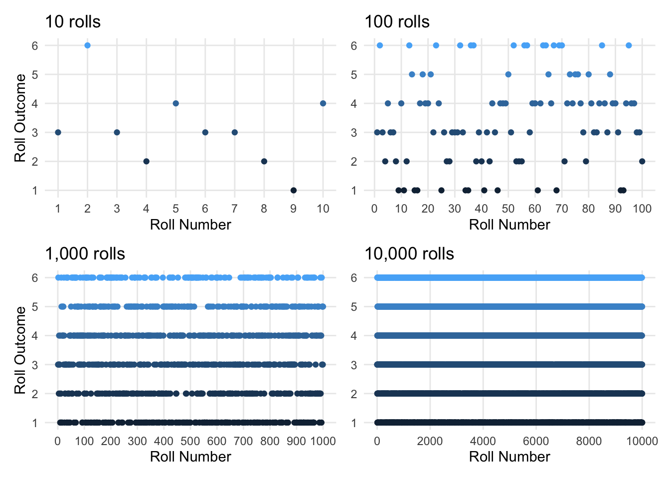
We again see that we didn’t roll a five in the first 10 rolls, but that three fives came up shortly thereafter. As we expand the number of rolls, we see that, despite frequent gaps, all numbers start to fill in. The more we roll, the closer the outcomes move to their expected probabilities.

Distribution of roll outcomes by number of total rolls:

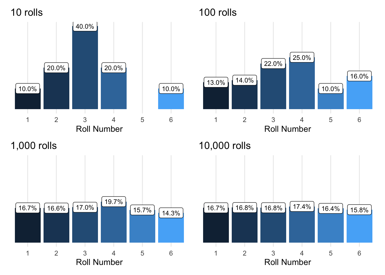
If we look at the distribution of outcomes at each of the stages, we see that with only ten rolls, most outcomes are far from their expected probabilities. Even at 100 it seems that 1, 2, and 5 are simply less likely.

But as we continue to roll, we observe these under-represented outcomes making a comeback. By 1,000 rolls, all outcomes are approaching their intrinsic probability values and by 10,000 rolls, it is closer still. This is a demonstration of the law of large numbers.

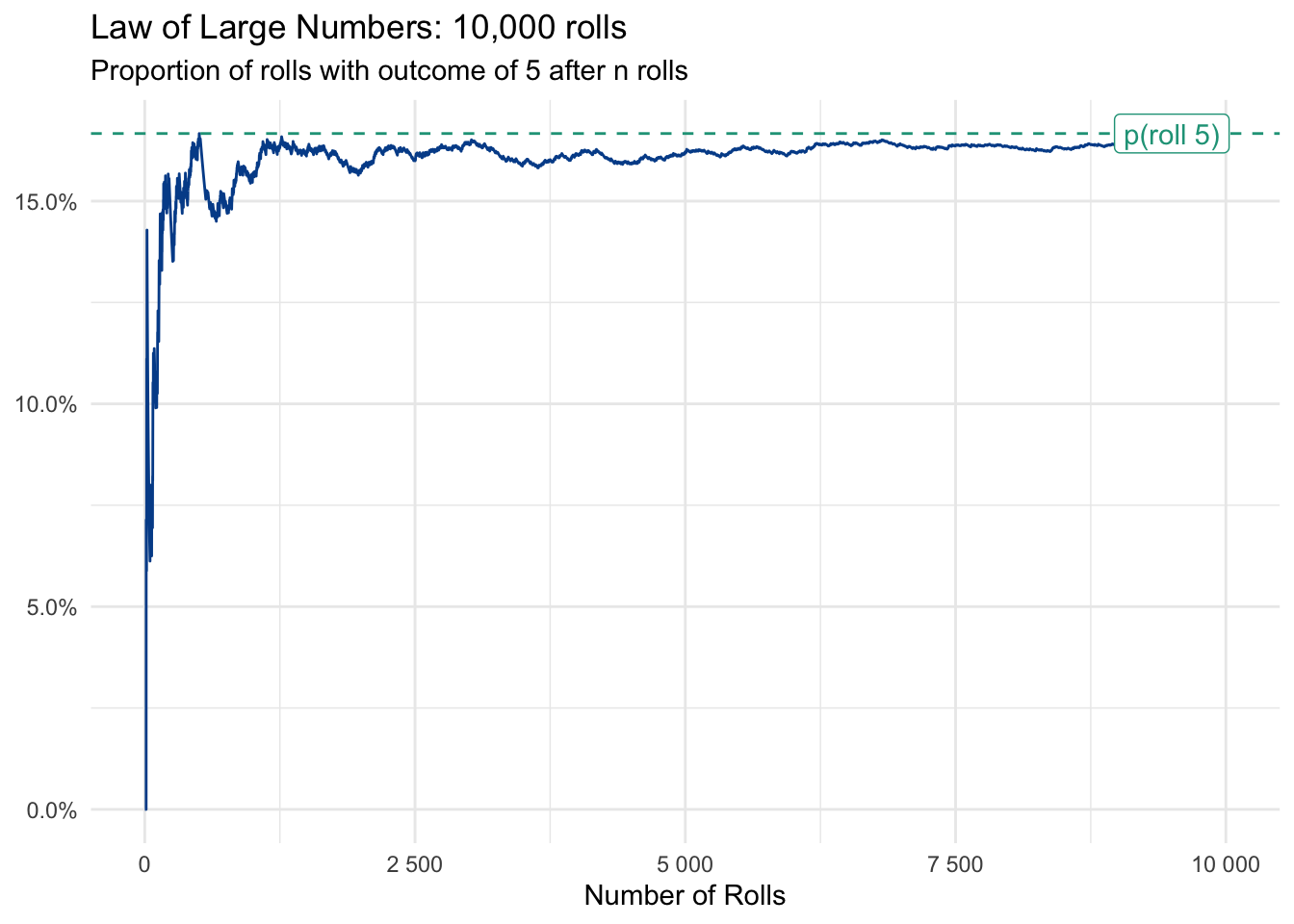
Although randomness in the early die rolls resulted in five coming up less than expected, the rate at which a five is thrown eventually approaches its calculated probability of 16.7% with enough rolls.

Customer purchases

The law of large numbers works beyond games of chance.

Let’s say you own an e-commerce platform that sells only one product, an electric lawnmower. History tells you that 1.27 percent of your web traffic ends up purchasing the product. Based on this conversion rate, a new manager may be surprised when none of the first 350 visitors to the site make a purchase. Is the payment system down? Are we getting new traffic with unqualified leads?

The product manager raises these concerns with you, and you reply, “Don’t worry, this happens occasionally”. Recall from above that the probability of something not happening is equal to one minus the probability of something happening. So, we know there is a 98.73 percent chance that no conversion will occur on any given web visit. You can raise that probability to a factor of 350 to estimate the chance that none of the first 350 visitors make a purchase.

\[\text{p(no purchase in first 350 visitors) = 0.9873}^\text{350} = \text{0.0114 or 1.1%}\]

Unlikely does not mean impossible. The new manager goes out to lunch and comes back to find the day’s first sale, from the 395th site visitor.

With more confidence in the conversion rate when applied to large volumes of traffic, the manager decides to use it to estimate how many new visitors the company must attract to hit the quarterly revenue targets. Time to get marketing on the phone.

10.3 Tree diagrams

We can model sequential events by exploring conditional probabilities, the likelihood of something occurring given that some other outcome has already occurred. When there aren’t too many events or potential outcomes, a tree diagram helps to visualize the concept.

The diagram will show a branch for each outcome in a series of events. If you multiply the probabilities along a given outcome path, you will find the probability of that specific sequence.

Simple example

Let’s say you flip a coin twice in a row. Since the flips are independent events — meaning the outcome of one will not impact the outcome of the other — the probability of flipping a head or tail is always 50% or 0.5.

Although these characteristics lead to relatively boring tree diagrams, they make it easy to follow the two event branches and map the four possible sequential outcomes with their cumulative or joint probabilities.

There are four possible sequential outcomes, each with the same joint probability of occurring.

Head then Head | Probability = 50% x 50% = 25%
Head then Tail | Probability = 50% x 50% = 25%
Tail then Head | Probability = 50% x 50% = 25%
Tail then Tail | Probability = 50% x 50% = 25%

A tree diagram becomes more illustrative when moving beyond coin flips or dice rolls.

Gracie’s lemonade stand

Gracie Skye is an ambitious 10-year-old. Each Saturday, she sells lemonade on the bike path behind her house during peak cycling hours. It is a lot of work to prepare the stand and bring the right quantity of ingredients, for which she shops every Friday after school for optimal freshness.

It didn’t take Gracie long to realize that weather has a huge impact on potential sales. Not surprisingly, people buy more lemonade on hot days with no rain than they do on cold, wet days. She has even estimated a demand equation based on temperature.

\[\text{Glasses of lemonade sold = -100 + (1.7 x temperature)}\]

When it rains, demand falls an additional 20 percent across the temperature spectrum.

To generate a more realistic view of her business, and to influence ingredient purchase decisions, Gracie collected historic data to better respond to weather conditions.

She finds:

Probability of no rain: p(no rain) = 0.72
Probability of rain: p(rain) = 0.28

Further, she discovers that the temperature fluctuates widely depending on if it rains or not.

Visualizing likely outcomes

Gracie translates these probabilities into a tree diagram to get a better sense of potential outcomes and their respective likelihoods. The most probable outcome is to have no rain and a temperature of 85°F. This has a probability of 0.396. The least likely outcome is rain with a temperature of 95°F (p=0.014).

Expected outcomes

With this information, Gracie can then revisit her demand function to calculate revenue, cost, and profit expectations for each scenario based on:

Selling price: $2.00 per glass
Cost of goods sold: $0.80 per glass

Next, we will define expected value to help Gracie construct a best estimate for her business outcomes.

Here you can find a spreadsheet with calculations for the tree diagram outcomes discussed above.

10.4 Expected value

We used tree diagrams to visualize the individual and joint probabilities for a series of events with specific outcomes. If there is a numeric value associated with each outcome, we can also calculate the expected value or payout from participating in the event.

Let’s say we have three possible outcomes with payout values of 1, 5, and 100 dollars. The likelihood of these outcomes is well defined with probabilities of 75%, 20%, and 5%, respectively. A tree diagram for the single branch event looks like this:

To calculate the expected value, we simply multiply the individual probabilities against their associated payouts and then add up all the respective results. Although our example only has three possible outcomes, you can use the following formula to calculate as many outcomes as you need.

\[\text{Expected value = (Prob 1 x value 1) + (Prob 2 x value 2) + ... (Prob n x value n)}\]

Applying this to our simple example:

In this case, assuming we played the game or scenario many times, we’d expect an average payout of $6.75. Expected values lead to interesting discussions and decisions, such as the most you’d be willing to spend to participate in such a game.

Depending on how many times you plan on playing and your appetite for risk/potential profit, you probably don’t want to spend more than $6.75 to participate as this is what you would expect, over time, to earn from playing the game.

Gracie’s business expectations

Gracie’s lemonade stand, which was introduced in tree diagrams, is more complex as it is a series of random events and has an expected payout in the form of total demand, which then flows into revenue, cost, and profit implications.

Not surprisingly, she earns the greatest profits on the hottest days with no rain and the lowest profits on the coldest days with rain. As a testament to her business model, there are no days — at least based on weather — where she would expect to lose money.

Although Gracie knows the business outcomes associated with each distinct weather possibility, she doesn’t have a single estimate that summarizes the typical day.

By using the approach defined above she can calculate the expected value for demand and then work through calculations for revenue (demand x the $2 selling price of lemonade), cost (demand x the $0.80 cost of ingredients for each cup), and profit (total revenue - total cost).

Taking the sum of all probabilities multiplied against their associated demand outcome, Gracie calculates the expected value for demand. She can then either (1) use that expected value to calculated expected revenue, cost, and profit or (2) add up the probability adjusted figures in the table.

Expected demand: 38.2
Expected revenue: $76.4
Expected cost: $30.56
Expected profit: $45.84

On a typical day, Gracie can expect to attract 38 customers and earn nearly 50 dollars in profit. Not bad for a ten-year-old.

Expected value is an extension of weighted average and we can use =SUMPRODUCT() in spreadsheets to find the results shown above.

10.5 Monte Carlo simulations

A simulation is an artificial reconstruction of an actual event or series of events. Simulations enable us to observe a full distribution of outcomes when we have a defined set of probabilities. The term is often used interchangeably with Monte Carlo simulations, named after the famous Monte Carlo Casino in Monaco.

If you run enough simulations, your average outcome will approach the expected value based on the law of large numbers. However, you will now also be able to calculate additional descriptive statistics — such as the standard deviation — to give you a better sense of likely outcomes and the potential risks associated with them.

When we rolled a die 10,000 times no one physically picked up a die, rolled it, and recorded the value. Instead we relied on computer software to take the defined probabilities — 50 percent chance of getting heads and 50 percent chance of getting tails. The function we wrote took these inputs or parameters and repeated the artificial die roll 10,000 times. The computer helped maintain accuracy for the repetitive task and didn’t get bored along the way. It was also much faster, taking less than a second.

Simulations become more valuable in complex, multi-staged situations in which series of probabilities lead to multiple outcomes.

Simulating Gracie’s lemonade stand business

We return to the lemonade stand example set up in the tree diagrams section. The weather — rain and temperature — follow random distributions and impact our customer demand function.

Instead of using expected value calculations for each potential output, we could also have simulated the events using the following approach:

Step 1. Generate one random number, random1, to determine if there is rain or no rain

If we let the computer select a random number from 1 to 100, we can use the result to pick a rain outcome. In our example, there is a 28 percent chance of rain and a 72 percent chance of no rain. We map the random number to the probabilities by establishing cutoff points. If the random number is 28 or less, the result in the simulation is rain. If the random number is more than 28, the result is no rain.

Simulation 1, Random Number 1 = 63 –> no rain

Step 2. Generate a second random number, random2, to determine the temperature

We again have the computer select a random number from 1 to 100. This step, because of the characteristics of the event we are describing, is more complex than just choosing rain or no rain. Recall that if there is rain, we have one set of probabilities to determine the temperature. If there is no rain, we have another set.

Simulation 1, Random Number 2 = 82 –> Temperature = 95 degrees

Now that we know the weather conditions for our first simulation, we can apply our demand function the same way as before and calculate the derivative business outcomes based on the per-glass selling price of $2.00 and the ingredient cost of 80 cents.

Our simulation repeats the process until we have created 1,000 simulations, which are shown in the table below and come from these spreadsheet calculations.

Interpretation

The average demand estimate from the thousand simulations is 37.5, very close to the expected value of 38.2 found previously. Let’s take a look at what matters most for Gracie’s business.

Using the expected value approach, we were able to determine the expected profit of $45.84. If we take the average profit from the simulations, we calculate $44.95.

This shows us that simulations can be a good approximation of the pure theoretical values. Simulations also provide us with something that expected value alone does not — the distribution of outcomes.

1,000 simulation outcomes for temperature, demand, and profit

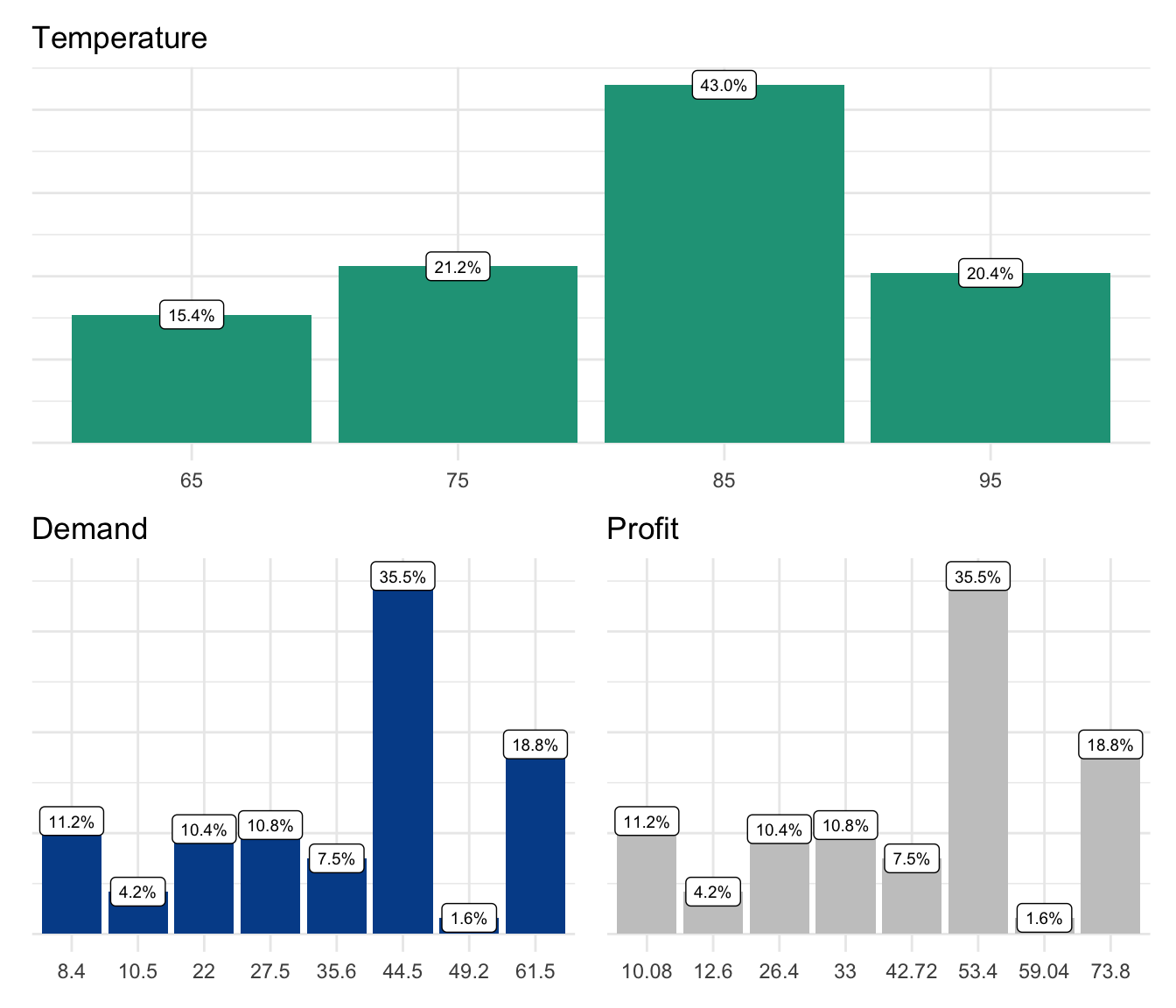
We get a clear sense from these 1,000 simulations what the distributed outcomes are likely to be. For instance, there is only a 20 percent chance that the temperature will be 95 degrees.

Looking at demand and profit, we see the exact same probabilities. This is because there are no random outcomes between demand and the purchasing behavior of buyers. We assume that all demand is satisfied. If we wanted to add more realism, we could say that revenue fluctuates up/down 10 percent depending on the negotiation skills of buyers at the lemonade stand.

Even the basic distributions are telling. We now see that there is a 56 percent chance that profit will be greater than 50 dollars. We could also use extreme values to make business decisions. For instance, if we only want to operate a business that generates more than 30 dollars in profit per day, we can use these results to highlight the 26 percent chance that profit will be less than 30 dollars on any given day. At some point, if the likelihood of those occurrences is too large or not offset by frequent days with much larger profits, we may decide to exit the business or not even enter in the first place.

Probability of x…

Another benefit that comes from simulations is the opportunity to apply an empirical cumulative distribution function to the results — something we’ll discuss more when looking at distribution types.

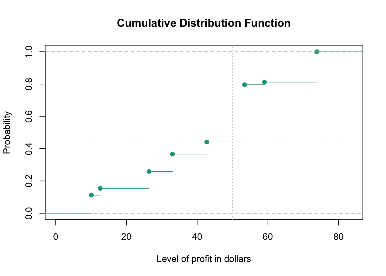
In essence, the plot shows the probability that Gracie will earn at least a given level of profit on a randomly selected day. For instance, there is a 44 percent chance that Gracie will earn at least 50 dollars in profit (shown at the intersection of the two dotted lines in the chart).