12 Generalizing results
Material in this section leans heavily on concepts defined in OpenIntro Statistics, a fantastic open-source statistics resource I’ve been teaching with since 2016.
12.1 Populations vs. samples
Life is made easy when the data at your disposal includes everything or everyone you care about.
If your customer tracking system is perfect, then the average sale is the actual average sale. If you speak to all potential voters, then the average opinion of an elected official is the actual average opinion.
In the real world, however, we are often limited to subsets or samples of data that come from a wider population. Because we don’t have all the information, we can’t be sure that our descriptive summaries precisely match reality.
Population
To illustrate this point, let’s use a modified Kaggle dataset from an e-commerce clothing store. It contains 23,486 purchase reviews from customers and includes age, a satisfaction rating from 1 (low) to 5 (high), and a short review. You can find the modified data here.
Let’s first assume that the store requires customers, at the time of purchase, to provide their age. The rating and review are requested at a later date, which explains the blank values for some of the rows.
Since we have data for every customer’s age, we can consider it the population and calculate the population mean from that data series as 43.2 years of age. Here is the distribution for all customers:
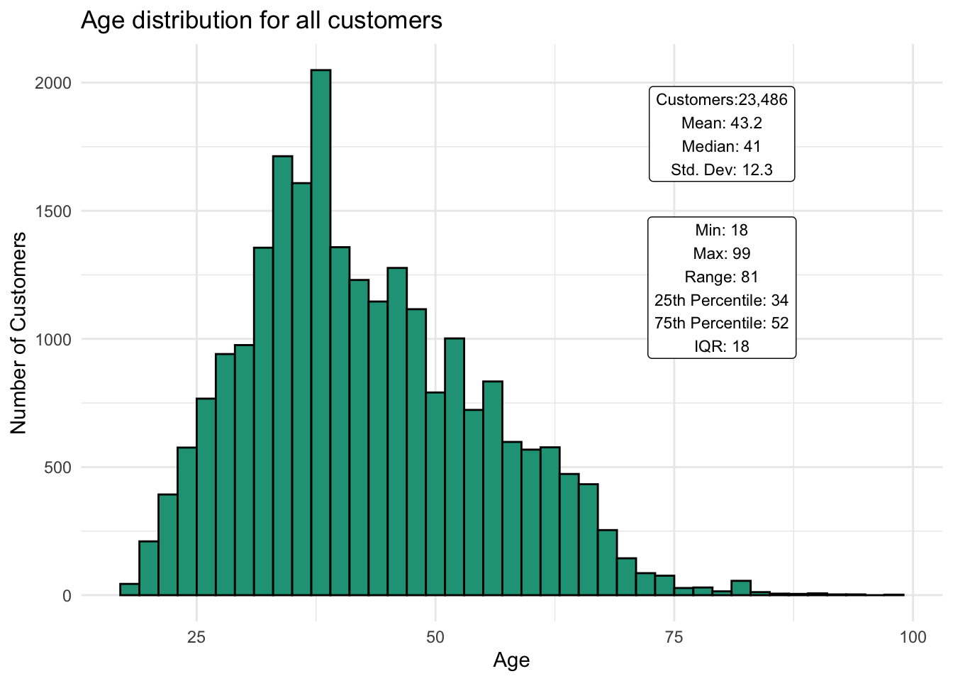
We have complete confidence in these summary statistics — as long as customers are being honest about their age!
Sample
Let’s now imagine that the same company didn’t collect customers’ ages at checkout and instead only asked in the follow-up survey.
In this case, the store would no longer know everyone’s age and have to rely on a smaller sample of people who happen to respond to the survey. The store’s manager knows that many people ignore survey requests and that sometimes invitations even end up in spam folders.
Based on experience, she only anticipates a one percent response rate. And one percent of 23,486 is only 235 people. How good could an age estimate be if she only hears from one percent of all customers?
The store manager runs the survey and ends up with a response rate of just 0.9 percent or 211 respondents. The mean age of survey respondents turns out to be 42.1. Remember, the store manager doesn’t have the full population mean of 43.2 to compare this against.
How confident can she be that the one number she has, the sample mean or point estimate for the population mean, is any good? Much of statistical theory is based on this type of question.
Measuring volatility
Imagine that the store manager was able to run the survey many times, reaching a different combination of random customers. How different might the sample mean be?
If she were to take 100 random samples from the known population, she would find the following sample means for age:
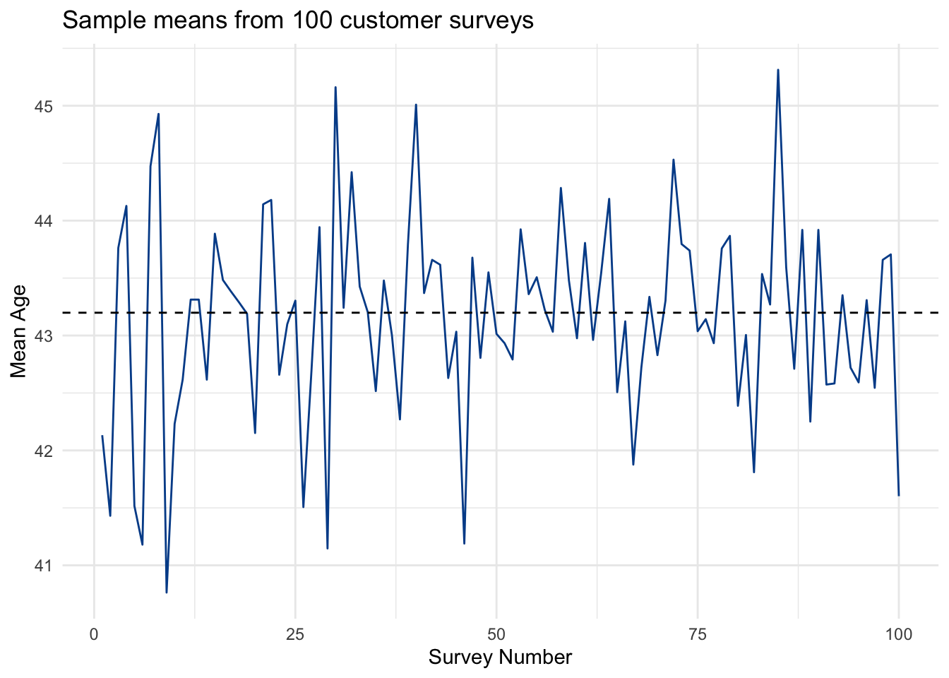
At first glance, this might look pretty noisy. But with the dashed line, which is the known population mean, you can start to see a pattern. Many of the sample means are close to that line, while every once in a while, we get an average that is off by one or two years of age.
This pattern is clearer when we look at sample means from the 100 surveys as a histogram.
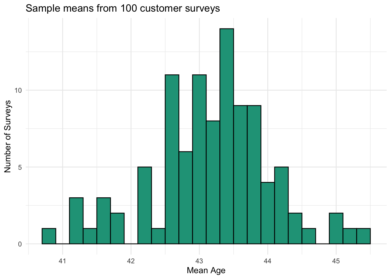
Although the full range of observed sample means for age fell between 40.8 and 45.3, most results were between 42 and 44.5. Considering that the age of customers in the full population range from 18 and 99, this is a fairly narrow window that might help us evaluate the accuracy of a given sample.
Watch what happens as we take the rolling average from each new set of survey results. With enough surveys, the mean age from the combined samples gets closer and closer to the known population value. Early variation is smoothed out as each new sample is more likely than not to be closer to the actual mean.
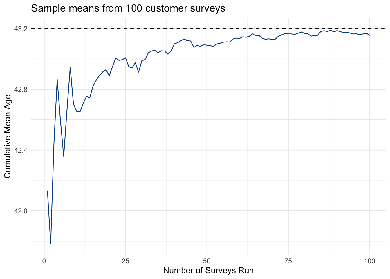
Although we are able to discern this convergence from a relatively small number of survey samples, imagine if we ran it 1,000 times.
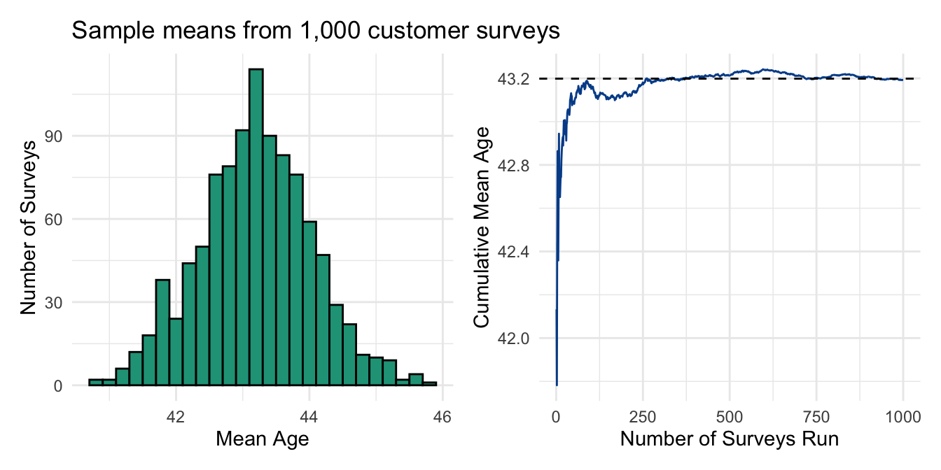
Now our histogram looks very much like a normal distribution and our rolling average continues to stay close to the true population mean.
Next, we’ll use this distribution and its characteristics to measure uncertainty with point estimates, which have come from samples of the population.
12.2 Standard errors
Sampling distribution
Let’s return to the mean age values from the 1,000 randomized surveys we administered to store customers. These point estimates represent the sampling distribution, a distribution that is approximately normal.
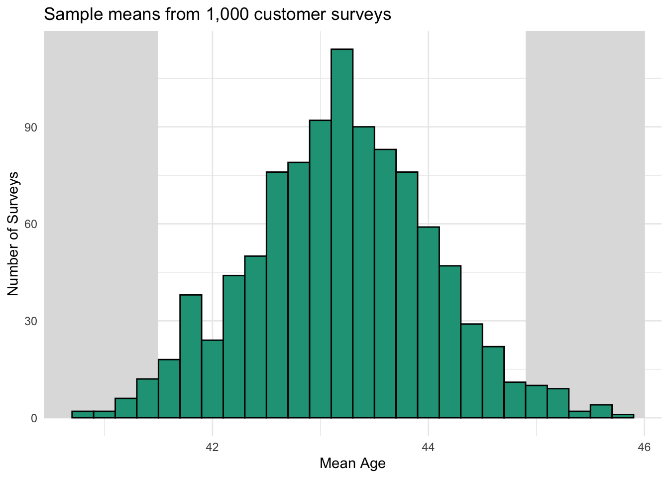
Although a small number of samples were found to have more extreme mean age estimates, the overwhelming majority (95%) came back between 41.5 and 44.9. The mean age from all samples, the sampling distribution, is 43.2, which matches exactly the mean age from the known population.
It is important to note that the distribution of the sample means is normal even though the distribution of ages from the entire population is not. This characteristic allows us to apply statistical techniques that work with normal distributions around such point estimates.
Standard error for a sample mean
We learned that standard deviation is a measure of spread among numbers in a data series. The standard deviation of all the sample means is 0.84, showing us how far, on average, a single sample mean is from the population mean. This standard deviation of a sampling distribution is also known as the standard error.
Recall that in our example we took 1,000 survey samples. In the real world, due to many considerations, we usually only take one sample, and the population metrics are unknown. This means that our one random sample could return a value anywhere along the distribution shown above.
We can use the standard error formula to find a measure of uncertainty from a single sample. Although the statistical proof uses the true population standard deviation as an input, the standard deviation from the individual sample also works as long as the sample size is sufficient because they will also be normally distributed.
\[\text{Standard error of mean (SE) = }\frac{\text{Sample standard deviation}}{\sqrt{n}}\]
Let’s now assume that (1) we don’t know the true population values and (2) we only administer one survey, which is our one sample. There are 211 respondents and we calculate a mean age of 42.13 with a standard deviation of 12.55. The standard error would be:
\[\text{SE = }\frac{\text{12.55}}{\sqrt{211}}= 0.8637\]
Standard error for a sample proportion
We can also calculate standard errors for proportions that are generated from samples. For instance, say we want to know the proportion of customer reviews that give five stars. Among people who provided a rating, these were the star distributions:
Now the question becomes, “How confident are we in the 54.6 percent estimate for the proportion of customers experiencing 5-star service?”
Standard errors for proportions relate to Bernoulli events, which have a probability of success, p. Here, we calculate the standard error as:
\[\text{Standard error of proportion (SE) = }\sqrt{\frac{p\times(1 - p)}{n}}\]
With our inputs:
\[\text{SE = }\sqrt{\frac{0.5459\times(1 - 0.5459)}{185}}= 0.0366 \text{ or 4%} \]
The standard errors for both mean age and the proportion of 5-star ratings reflect measures of uncertainty around these point estimates, which can be used to more explicitly quantify confidence in them.
12.3 Confidence intervals
12.3.1 One sample
We’ve seen that, with enough random observations, a point estimate such as the sample mean is likely to be relatively close to the population mean. However, it is very unlikely to match it exactly. To help measure this uncertainty, we can calculate confidence intervals for a given point estimate by leveraging the standard error.
Confidence interval for a sample mean
Calculating a confidence interval results in two values. A lower bound and an upper bound. Each is determined by taking the point estimate of the sample and then adding/subtracting 1.96 times the standard error.
\[\text{Confidence interval = Sample mean} \pm 1.96 \times \text{Standard error}\]
This calculates a 95 percent confidence interval due to the 1.96 input value that we’ll explain later. Plugging in values from our one sample:
\[\text{Confidence Interval = 42.13} \pm 1.96 \times \text{0.8637} = \text{40.4 to 43.8}\]
The result indicates that we are 95 percent confident that the actual population age mean is somewhere between 40.4 and 43.8 years of age.
Notice that these two points sit equal distance from our sample mean. The standard error is driven by the standard deviation of observed sample values. A larger standard deviation will therefore result in wider confidence intervals (less certainty) and a smaller one will result in tighter intervals (more certainty).
The 95 percent confidence statement also indicates that if we took 100 samples, 95 out of 100 times we would expect our confidence interval to contain the true population mean — as it does in our one sample illustration.
Spreadsheets calculations can be found here.
Confidence interval for a sample proportion
When dealing with sample proportions, the formula remains the same.
\[\text{Confidence interval = Sample proportion} \pm 1.96 \times \text{Standard error}\]
The difference comes from the standard error calculation, which we calculated above as 0.0366 based on the proportion of 5-star reviews (0.5459) from the 185 records that provided a rating.
\[\text{Confidence interval = 0.5459} \pm 1.96 \times \text{0.0366} = \text{0.4742 to 0.6176}\]
Here, we are 95 percent confident that the true population proportion of 5-star reviews falls between 47.4% and 61.8%.
Why do we use 1.96?
Remember the 68-95-99.7 rule? It stated that a normal distribution will have a certain percent of its observations fall within one, two, and three standard deviations from the mean.
We can standardize values within a data range based on their distance from the mean. This is referred to as a standardized score or z-score for each observation. Larger values will have positive z-scores, reflecting their relative distance above the mean. The same is true in reverse for smaller values.
\[\text{Standardized z-score =}\frac{(\text{Observed value - Mean value})}{\text{Standard deviation}}\]
Applying this transformation to the sample means from the sampling distribution moves us from the chart on the left to the chart on the right, which is now centered around a mean of zero and standard deviation of one.
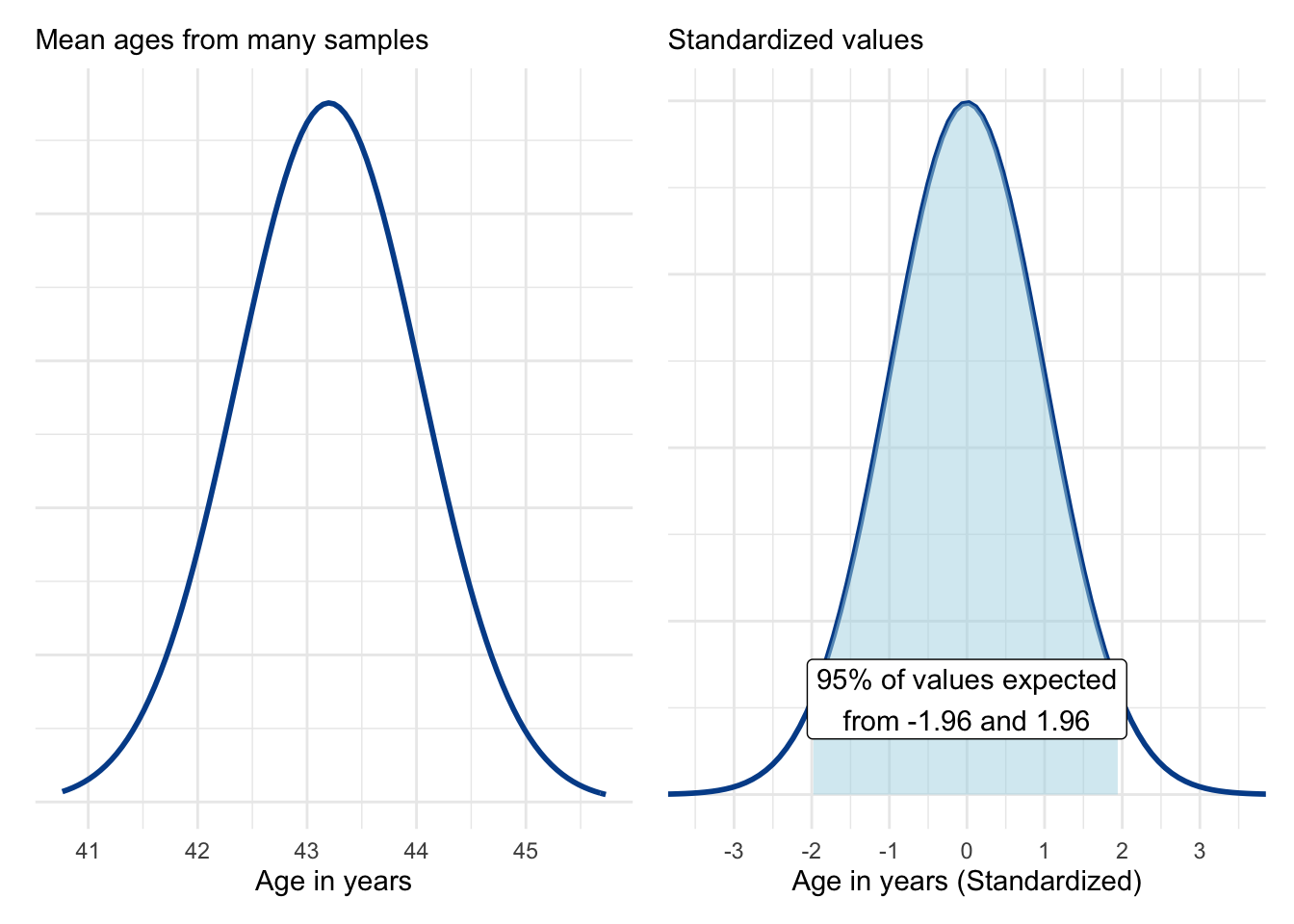
We can see that within a normal distribution, 95 percent of values are expected to fall from a z-score value of negative 1.96 to positive 1.96. Because the sampling distribution is normal, we know that if we take just one sample, there is a 95 percent chance its value will be within the range shown above.
Different levels of confidence
If we want to be more confident, we have to make the shaded area larger by selecting a larger z-score cutoff value. This would increase the size of our confidence intervals. In other words, to be more confident, we need to allow for more potential values or deviations from the mean.
If we are okay with a lower level of confidence, our confidence interval ranges will get smaller. The 95 percent confidence interval is most common in practice. But in situations where potential errors are more costly, it may be increased to 99 percent confidence levels or higher. You generally will not see people using confidence intervals below 90 percent.
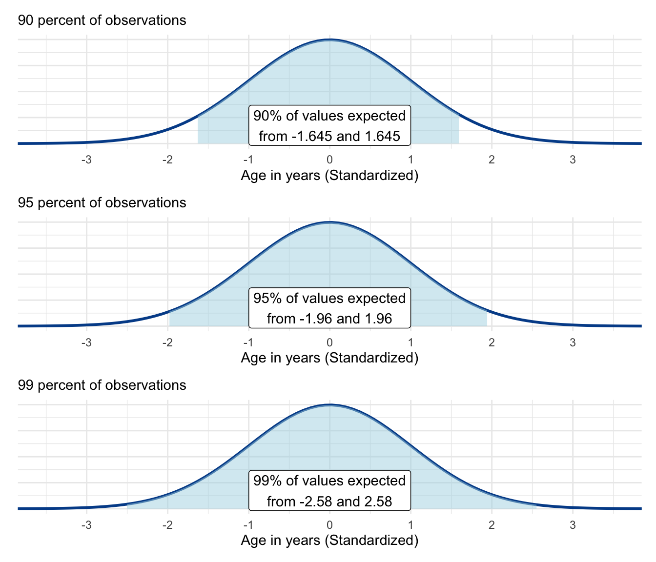
These visuals illustrate cutoff values for 90, 95, and 99 percent confidence levels. Of course, they are arbitrary, and any potential confidence level could theoretically be selected based on various z-score cutoffs.
Confidence intervals are a great tool to communicate uncertainties in analysis that is based on samples of data from a wider population. They can also help us identify if meaningful differences exist between two samples or among different groups within the same sample.
12.3.2 Two samples
With confidence intervals, we were able to express our level of confidence with a given point estimate, such as a mean derived from one sample. However, a common data task is to make judgments on significant differences between groups.
Let’s revisit our sample from the customer reviews dataset, splitting the star ratings by the 135 people younger than 50 and the 50 people who happen to be 50 and older.
It appears that younger people are more likely (56.3%) than older people (50.0%) to provide 5-star ratings. But once again, how much confidence do we have in this apparent difference?
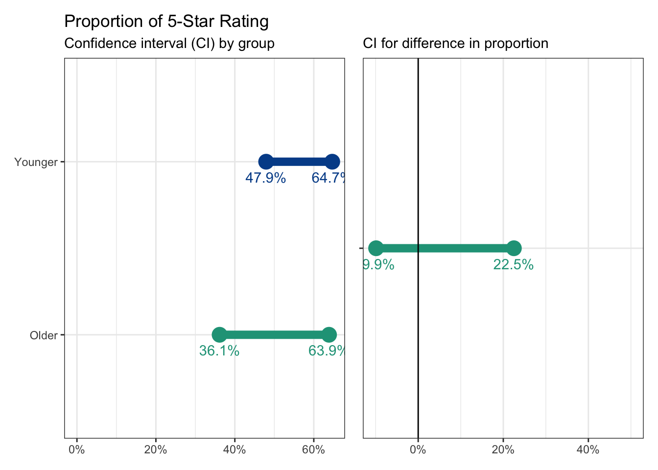
The number of observations and measures of standard error will help us gain clarity. And if we treat both groups as their own samples, we can calculate respective confidence intervals as before, leading to these results:
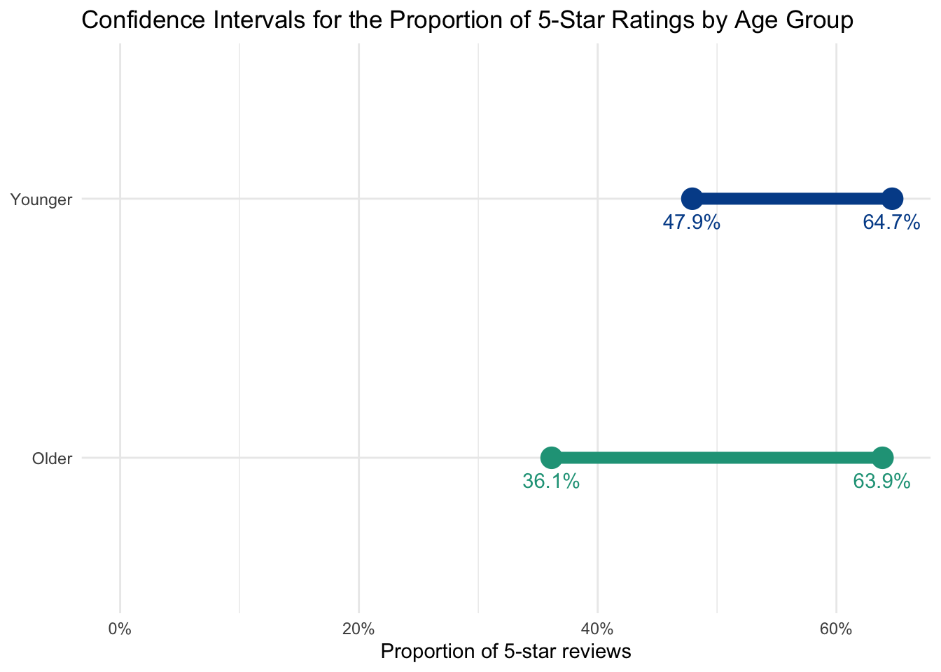
We are 95 percent confident that the true proportion of 5-star ratings for younger people ranges from 47.9% to 64.7%. This is a smaller range than for older customers (36.1% to 63.9%) largely due to a smaller number of older respondents in the sample. When confidence intervals overlap, as they do in our visual, it is very likely that we don’t have enough evidence to declare statistically significant differences between the groups.
Confidence interval for the difference between two proportions
Another way to look at the problem is to focus on the observed differences and calculate one set of confidence intervals that unifies both groups. Here, the formula gets more complex. The standard error portion of the calculation incorporates summary information from both sample 1 and sample 2:
\[\text{Confidence interval for difference between two proportions = }\]
\[p1-p2\pm1.96\times\sqrt{\frac{p1\times(1 - p1)}{n1}+\frac{p2\times(1 - p2)}{n2}}\]
Plugging in values from our example, using 1 for younger customers and 2 for older ones:
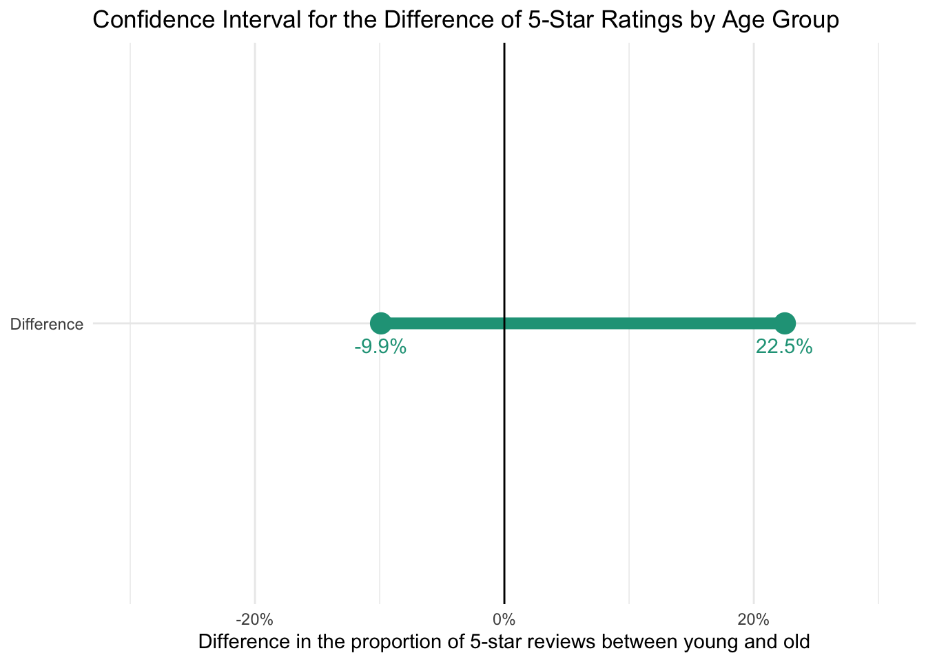
\[0.563-0.5\pm1.96\times\sqrt{\frac{0.563\times(1 - 0.563)}{135}+\frac{0.5\times(1 - 0.5)}{50}}=\] \[\text{-0.0989 to 0.2249}\]
The resulting values show a 95 percent confidence that the true population proportional differences between 5-star selection by young and old people is between -9.9% and 22.5%. As long as this range includes both negative and positive values, we will not be confident that significant differences exist.
These calculations can be found here.
Statistical significance
Confidence intervals only take us so far in determining statistical significance. When two confidence intervals don’t overlap or there are only positive or only negative values when looking at proportions, we know that the differences are statistically significant.
If they do overlap or if the difference in proportions has both positive and negative values along its confidence interval, then we’re not ready to make a formal declaration. For this’ we’ll turn to the concept of p-values.
12.4 Statistical significance
We compared two proportions from different survey groups and found that the confidence interval for their difference included negative and positive values, not a great indication that the differences are statistically different. Formal significance testing is required, however, to make a formal declaration.
The scientific method
Science is all about finding new evidence that makes us comfortable moving beyond previously held beliefs. Hypothesis testing is the widely adopted process for this. It states two positions: a null hypothesis that generally reflects a prevailing view and an alternative hypothesis to be tested.
We analyze data to determine if there is enough evidence to reject the null hypothesis in favor of the new, alternative one. Subsequent rounds of scientific inquiry will then test against any newly established belief.
Hypothesis testing
In the context of the 5-star review differences among younger and older customers, we can frame the problem as follows:
- Null hypothesis: There is no difference in 5-star rating behavior between young and old customers.
- Alternative hypothesis: There is a difference in 5-star rating behavior between young and old customers.
Translating these positions into numbers, the null hypothesis would have the true proportion of 5-star ratings be equal for both groups, p1 = p2. The alternative would be that the true proportions are different, p1 ≠ p2. Because uncertainty exists from the samples we’ve taken, significance testing is the formal method to evaluate if observed differences are statistically significant or not.
Recall our 95 percent confidence intervals for proportional differences between 5-star ratings by young and old people.
Significance testing
Although getting beyond the scope of data literacy, some of you may wish to see the steps that lead to a formal declaration of statistical significance. We will therefore run a z-test on the difference between two observed proportions. We need a single proportion and standard error to generate the expected sampling distribution and will focus on observations from both groups to do so.
Step 1: Come up with a pooled proportion from the sample
\[\text{Pooled proportion (p) =}\frac{\text{(p1 * n1) + (p2 * n2)}}{\text{n1 + n2}}=\] \[\frac{\text{(0.563 * 135) + (0.5 * 50)}}{\text{135 + 50}}= 0.546\]
Step 2: Calculate a standard error
\[\text{Standard error = }\sqrt{p\times(1 - p)\times(\frac{1}{n1}+\frac{1}{n2})}=\] \[\sqrt{0.546\times(1 - 0.546)\times(\frac{1}{135}+\frac{1}{50})}=0.0824\]
Step 3: Determine a z-score which will be our test statistic
\[\text{Z-score} = \frac{(p1 - p2)}{\text{Standard error}}=\frac{0.563 - 0.5}{0.0824}= 0.7645631\]
This value serves as our cutoff point for the theoretical distribution of possible sample observations. We want to calculate the percent of these values above 0.7645631 and below -0.7645631, which will determine our p-value used to make a statistical significance conclusion.
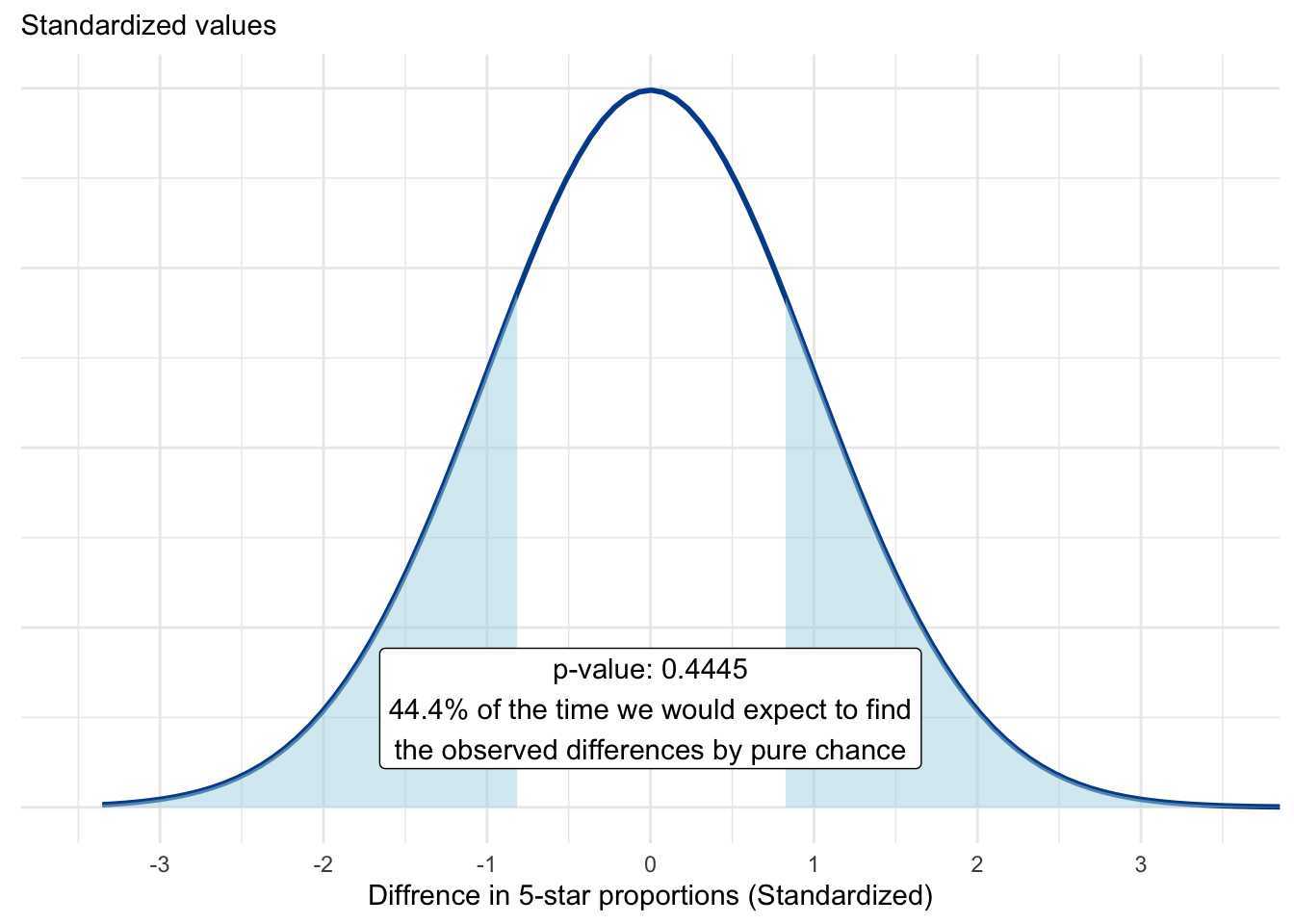
What does this show? The higher the p-value, the greater probability that our observed differences are due purely to chance. In this case, that level is nearly 50 percent, which is a lot of uncertainty that leads us to fail to reject the null hypothesis, meaning we haven’t found enough evidence to determine a meaningful proportional difference between the groups.
If we want to be 95 percent confident that the observed proportional difference is real, we will require a p-value of less than 0.05 or 5 percent.
These calculations can be found here.
An example of statistical significance
Let’s keep our sample size the same but adjust the proportion of 5-star ratings for each group to 65% for younger customers and 45% for older customers. On the surface, this appears like a large difference, but remember it is still based on a sample and the sample has a relatively small number of respondents in each group.
Here are the confidence intervals associated with the new proportions.
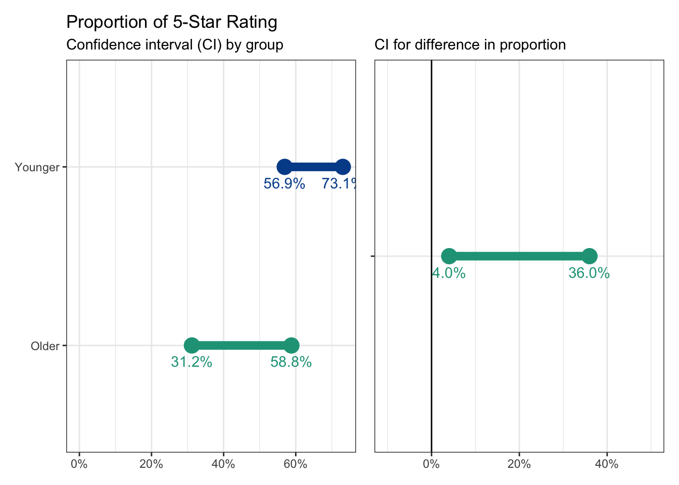
We mentioned previously that we won’t be able to determine significance if the individual confidence intervals are overlapping. Here, there is still slight overlap for each group, although the confidence interval for the proportional difference now only has positive values.
Let’s follow the steps to find a p-value, from which we can make a significance decision.
Step 1: Come up with a pooled proportion from the sample
\[\text{Pooled proportion (p) =}\frac{\text{(p1 * n1) + (p2 * n2)}}{\text{n1 + n2}}=\] \[\frac{\text{(0.65 * 135) + (0.45 * 50)}}{\text{135 + 50}}= 0.5959\]
Step 2: Calculate a standard error
\[\text{Standard error = }\sqrt{p\times(1 - p)\times(\frac{1}{n1}+\frac{1}{n2})}=\] \[\sqrt{0.5959\times(1 - 0.5959)\times(\frac{1}{135}+\frac{1}{50})}=0.0812\]
**Step 3: Come up with a z-score which will be our test statistic
\[\text{Z-score} = \frac{(p1 - p2)}{\text{Standard error}}=\frac{0.65 - 0.45}{0.0812}= 2.4630542\]
This value was used as a cutoff for our theoretical distribution of proportional differences.
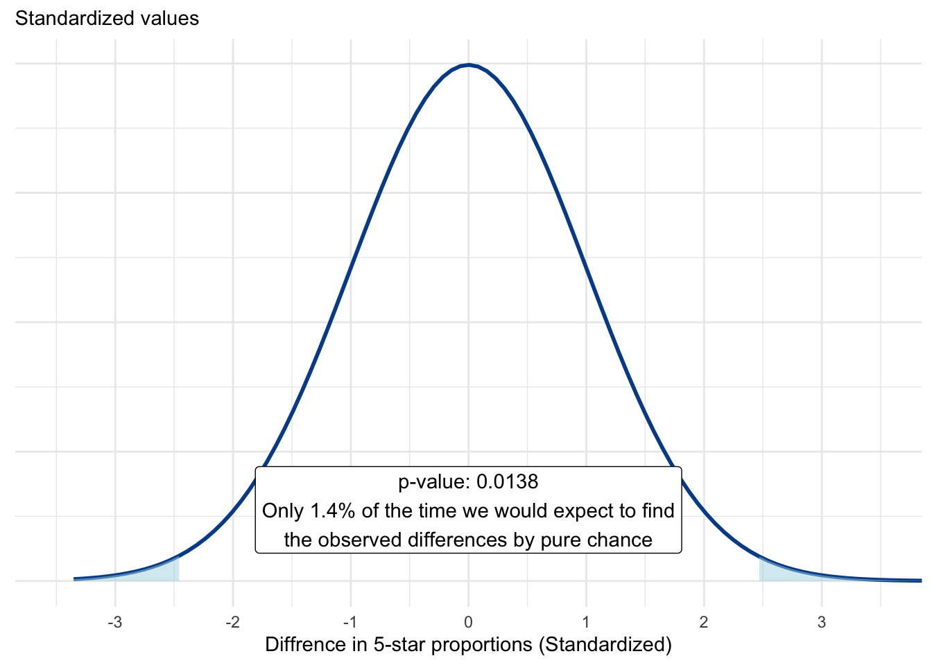
Now we see a lot less shaded area in our plot, only 1.4 percent. This indicates a much lower probability that our observed differences from the samples are due to chance. Not impossible, but highly unlikely.
We now have the evidence we need to declare with 95 percent confidence that our observed proportional differences are statistically significant. We reject the null hypothesis in favor of the alternative hypothesis. There is a meaningful proportional difference and younger customers appear more likely to give 5-star reviews than older customers.
This is just one example of statistical significance testing and there are many more depending on the type of data and the hypothesis in question. If you are interested in learning more, I suggest starting with this article from Towards Data Science.