
Tree diagrams in R
June 28, 2020A tree diagram can effectively illustrate conditional probabilities. We start with a simple example and then look at R code used to dynamically build a tree diagram visualization using the data.tree library to display probabilities associated with each sequential outcome.
You can find the single-function solution on GitHub.
Gracie’s lemonade stand
Gracie Skye is an ambitious 10-year-old. Each Saturday, she sells lemonade on the bike path behind her house during peak cycling hours. It is a lot of work to prepare the stand and bring the right quantity of ingredients, for which she shops for every Friday after school for optimal freshness.
It didn’t take Gracie long to realize that weather has a huge impact on potential sales. Not surprisingly, people buy more lemonade on hot days with no rain than they do on wet, cold days. She has even estimated a demand equation based on temperature.
Glasses of Lemonade =−100+1.7×Temperature
When it rains, demand falls an additional 20% across the temperature spectrum. To generate a more realistic view of her business, and to inform ingredient purchasing decisions, Gracie collected historic data to help her better anticipate weather conditions.
She finds:
- Probability of rain: p(rain) = 0.72
- Probability of no rain: p(no rain) = 0.28
Further, she knows the temperature fluctuates widely depending on if it rains or not.
| Temperature | No rain | Rain |
|---|---|---|
| 95°F | 0.25 | 0.05 |
| 85°F | 0.55 | 0.25 |
| 75°F | 0.15 | 0.35 |
| 65°F | 0.05 | 0.35 |
Visualizing likely outcomes
Gracie translates these probabilities into a tree diagram to get a better sense of all potential outcomes and their respective likelihoods. The most probable outcome is to have no rain and a temperature of 85°F. There is a probability of 0.396 associated with this. The least likely outcome is rain with a temperature of 95°F (p=0.014).
Expected outcomes
She then uses her demand function to calculate revenue, cost, and profit expectations for each scenario based on:
- Selling price: $2 per glass
- Cost of goods sold: $0.8 per glass
| Temperature | Rain | Prob | Demand | Revenue | Cost | Profit |
|---|---|---|---|---|---|---|
| 85 | no rain | 0.396 | 44 | 88 | 35.2 | 52.8 |
| 95 | no rain | 0.18 | 62 | 124 | 49.6 | 74.4 |
| 75 | no rain | 0.108 | 28 | 56 | 22.4 | 33.6 |
| 75 | rain | 0.098 | 22 | 44 | 17.6 | 26.4 |
| 65 | rain | 0.098 | 8 | 16 | 6.4 | 9.6 |
| 85 | rain | 0.07 | 36 | 72 | 28.8 | 43.2 |
| 65 | no rain | 0.036 | 10 | 20 | 8 | 12 |
| 95 | rain | 0.014 | 49 | 98 | 39.2 | 58.8 |
Taking the sum of all probabilities multiplied against their associated business outcome, Gracie calculates expected values for revenue, cost, and profit for her lemonade stand operations.
- Expected Revenue: $76.23
- Expected Cost: $30.49
- Expected Profit: $45.74
Making tree diagrams in R
I created this example because there don’t seem to be many r packages with flexible outputs for tree diagrams. Specifically, I needed something with the ability to:
- Take individual probabilities as inputs
- Calculate and display the joint or cumulative probabilities for each potential outcome
The solution was to use the data.tree package and build the tree diagram with custom nodes.
Load the probability data
All that is required is two columns:
- pathString: This defines how the tree should be structured. In our example, the first branch level is rain or no rain. To add a second branch of decisions or possible paths, simply add the outcome to the first branch name with a
/separator. For instance,rain/95°F, indicates the outcome of rain and a temperature of 95 degrees. The name of this variable, pathString, is important because it is expected by theas.Node()function we’ll call later. - prob: The probability associated with a specified event.
Let’s load in our input data from which we want to create a tree diagram.
prob_data <- read_csv("https://docs.google.com/spreadsheets/d/e/2PACX-1vQWc07o1xTNCJcGhw-tWYAnD3xPCjS0_jE4CIBR-rp5ff3flVGJQf2K24bJ5FE-DauQvLrtB8wWJNuc/pub?gid=0&single=true&output=csv")| pathString | prob |
|---|---|
| no rain | 0.72 |
| no rain/95°F | 0.25 |
| no rain/85°F | 0.55 |
| no rain/75°F | 0.15 |
| no rain/65°F | 0.05 |
| rain | 0.28 |
| rain/95°F | 0.05 |
| rain/85°F | 0.25 |
| rain/75°F | 0.35 |
| rain/65°F | 0.35 |
Create some helper variables
The goal in this step is to generate some new variables from the original inputs that will help define the required tree structure.
- tree_level: the branch level on a tree for a specific probability.
- tree_group: the name of the first branch to lookup parent probabilities
- node_type: a unique name to build custom components in the visualization
We also make a variable named max_tree_level that tells us the total number of branch levels in our tree.
prob_data <- prob_data %>%  mutate(tree_level = str_count(string = pathString, pattern = "/") + 1,
         tree_group = str_replace(string = pathString, pattern = "/.*", replacement = ""),
         node_type = "decision_node"
  )

max_tree_level <- max(prob_data$tree_level, na.rm = T)
Finding parent probabilities
For us to determine the cumulative probability for a given outcome, we need to multiply the probabilities in secondary branches against the probability of the associated parent branch.
To do this, we create a new data frame, parent_lookup, that contains all probabilities from our input source. We then loop through the tree levels, grabbing the probabilities of all parent branches. Finally, we calculate the cumulative probability overall_prob by multiplying across all probabilities throughout a branch sequence.
parent_lookup <- prob_data %>% distinct(pathString, prob) # get distinct probabilities to facilitate finding parent node probability

for (i in 1:(max_tree_level -  1)) { # loop through all tree layers to get all immidiate parent probabilities (to calculate cumulative prob)

  names(parent_lookup)[1] <-paste0("parent",i)
  names(parent_lookup)[2] <-paste0("parent_prob",i)

  for (j in 1:i) {

    if (j == 1)  prob_data[[paste0("parent",i)]] <- sub("/[^/]+$", "", prob_data$pathString)
    else if (j  > 1) prob_data[[paste0("parent",i)]] <- sub("/[^/]+$", "", prob_data[[paste0("parent",i)]])
  }

  prob_data <- prob_data %>% left_join(parent_lookup, by = paste0("parent",i))

}


prob_data$overall_prob <- apply(prob_data %>% select(contains("prob"))  , 1, prod, na.rm = T)  # calculate cumulative probability
Generating terminal nodes
For us to display the final probability on the tree diagram, we will need to pass data from a node_type named terminal. Because we need unique pathString values, we do this by replicating the final branch probabilities (along with the cumulative probabilities we calculated above) and adding /overall to the pathString.
The final steps are to:
- add the terminal rows back to the
prob_datadata frame - add one last row, with tree_level 0, that is the starting point for the tree. Here we name this
weatherfor itspathString.
terminal_data <- prob_data %>%  filter(tree_level == max_tree_level) %>% # create new rows that will display terminal/final step calulcations on the tree
  mutate(node_type = 'terminal',
         pathString = paste0(pathString, "/overall"),
         prob = NA,
         tree_level = max_tree_level + 1)

start_node <- "weather" # name the root node

prob_data = bind_rows(prob_data, terminal_data) %>%  # bind everything together
  mutate(pathString = paste0(start_node,"/",pathString),
         overall_prob = ifelse(node_type == 'terminal', overall_prob, NA),
         prob_rank = rank(-overall_prob, ties.method = "min", na.last = "keep"))

prob_data = bind_rows(prob_data, data.frame(pathString = start_node, node_type = 'start', tree_level = 0)) %>% # add one new row to serve as the start node label
  select(-contains("parent"))
Our final data frame, prob_data, is now ready to be passed to a visualization function.
| pathString | prob | tree_level | tree_group | node_type | overall_prob | prob_rank |
|---|---|---|---|---|---|---|
| weather | 0 | start | ||||
| weather/no rain | 0.72 | 1 | no rain | decision_node | ||
| weather/rain | 0.28 | 1 | rain | decision_node | ||
| weather/no rain/95°F | 0.25 | 2 | no rain | decision_node | ||
| weather/no rain/85°F | 0.55 | 2 | no rain | decision_node | ||
| weather/no rain/75°F | 0.15 | 2 | no rain | decision_node | ||
| weather/no rain/65°F | 0.05 | 2 | no rain | decision_node | ||
| weather/rain/95°F | 0.05 | 2 | rain | decision_node | ||
| weather/rain/85°F | 0.25 | 2 | rain | decision_node | ||
| weather/rain/75°F | 0.35 | 2 | rain | decision_node |
Visualization function
We make a function, make_my_tree, that takes a data frame with columns PathString and prob and returns a tree diagram along with the conditional probabilities for each path. The function can handle three additional arguments:
- display_level: Enables us to control how many branches of the tree diagram to display. The default is NULL which will show the entire tree.
- show_rank: Option to show the rank of the final probability along with the terminal node. The default is FALSE where the rank is not shown.
- direction: Option to change the direction that the tree is show. Default is
LRor left to right.RLwill display the tree right to left. Any other value with show it top-down.
make_my_tree <- function(mydf, display_level = NULL, show_rank = FALSE, direction = "LR") {

  if (!is.null(display_level) ) {
    mydf <- mydf %>% filter(tree_level <= display_level)

  }

  mytree <- as.Node(mydf)

  GetEdgeLabel <- function(node) switch(node$node_type, node$prob)

  GetNodeShape <- function(node) switch(node$node_type, start = "box", node_decision = "circle", terminal = "none")


  GetNodeLabel <- function(node) switch(node$node_type,
                                        terminal = ifelse(show_rank  == TRUE, paste0("Prob: ", node$overall_prob,"\nRank: ", node$prob_rank),
                                                          paste0("Prob: ", node$overall_prob)),
                                        node$node_name)

  SetEdgeStyle(mytree, fontname = 'helvetica', label = GetEdgeLabel)

  SetNodeStyle(mytree, fontname = 'helvetica', label = GetNodeLabel, shape = GetNodeShape)

  SetGraphStyle(mytree, rankdir = direction)

  plot(mytree)

}
Show the decision tree
Passing our data frame to the make_my_tree produces this baseline visual.
make_my_tree(prob_data)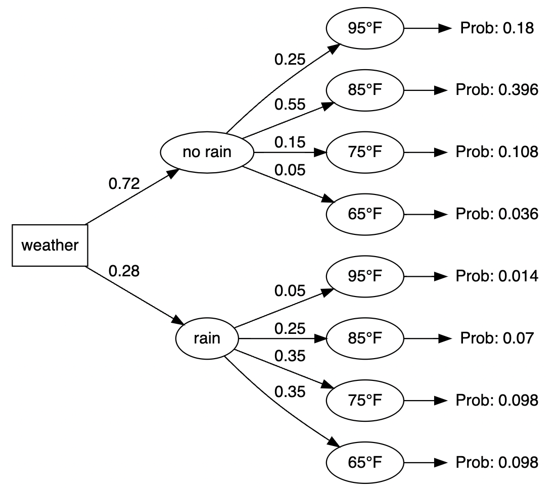
Alternative outputs
And here are a few alternative versions based on the optional arguments we included in the make_my_tree function.
Only the first branch
make_my_tree(prob_data, display_level = 1)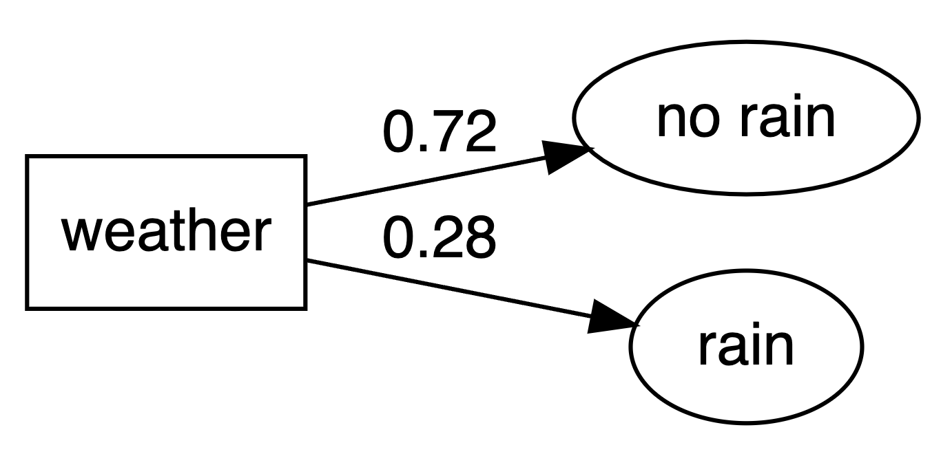
Full tree without the conditional probabilities
make_my_tree(prob_data, display_level = 2)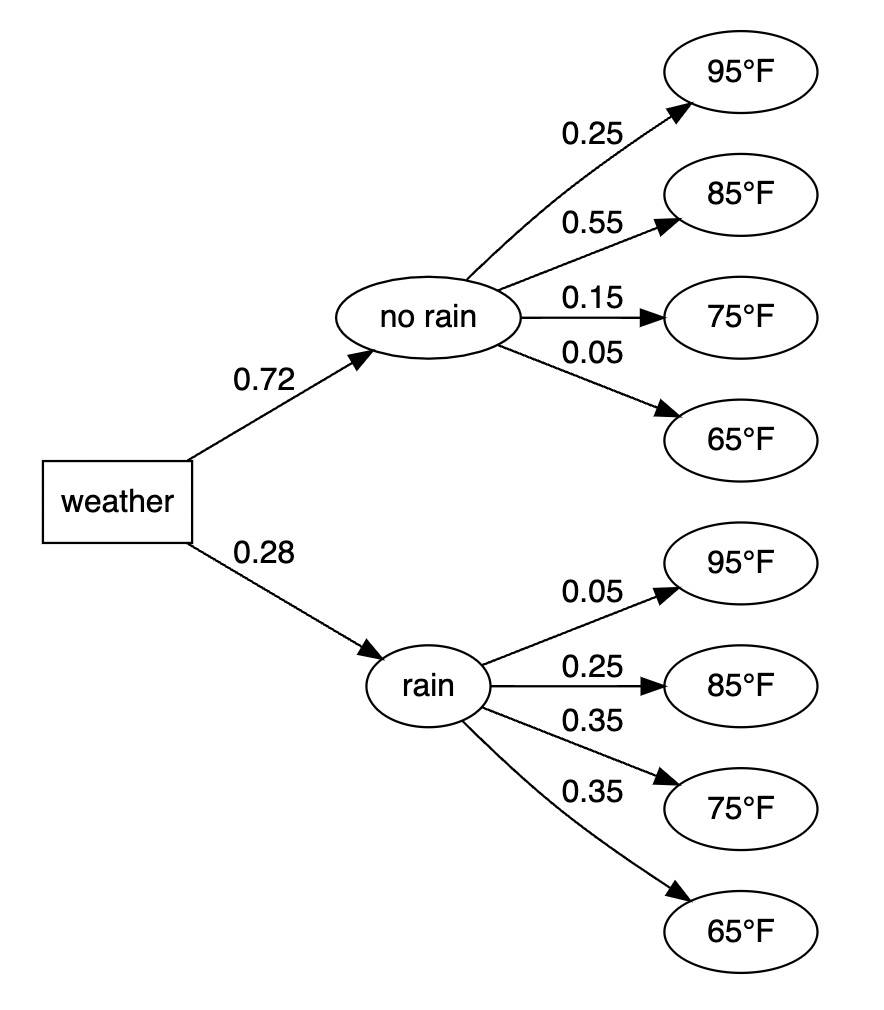
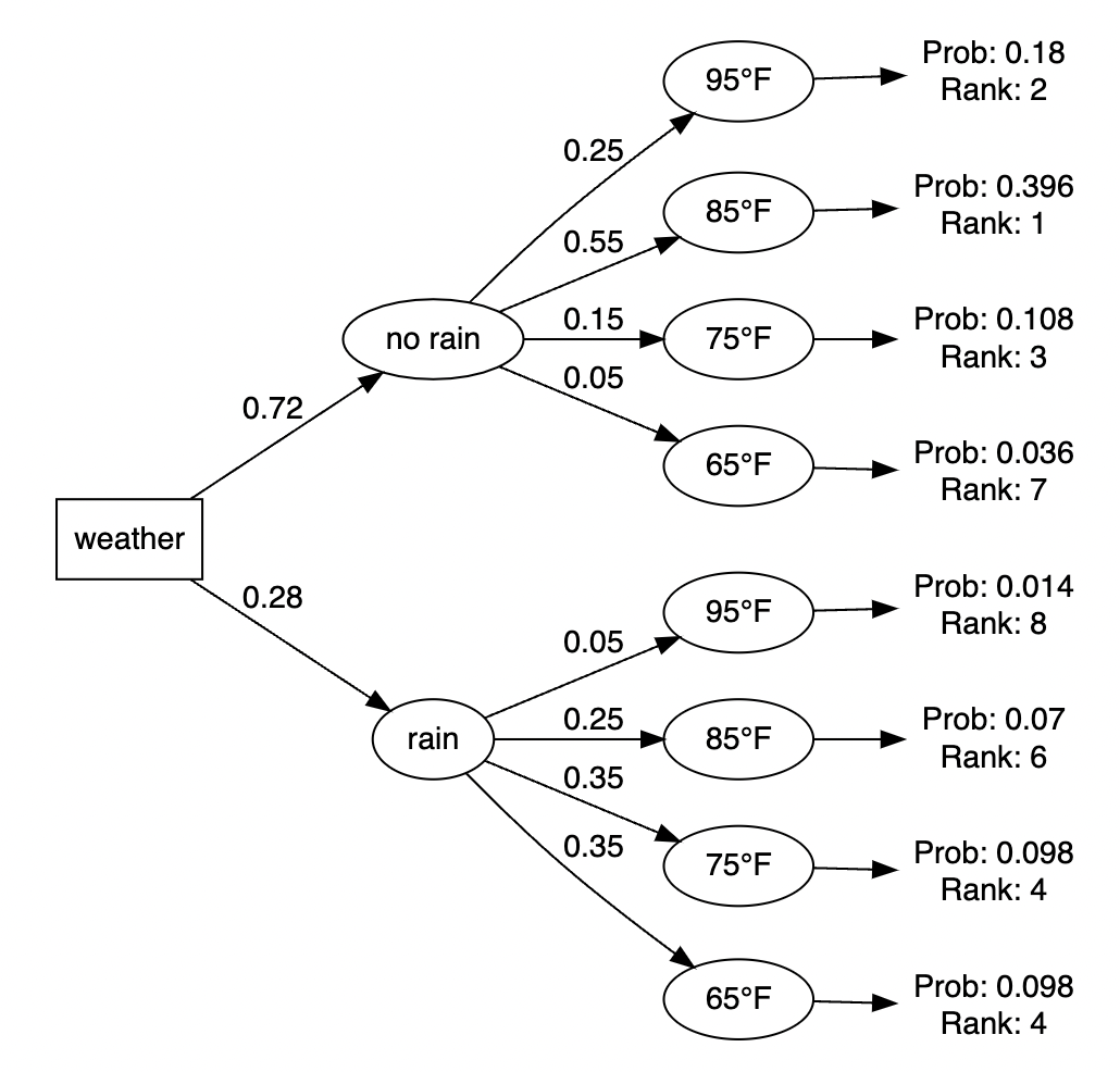
Everything including ranks
make_my_tree(prob_data, show_rank = TRUE)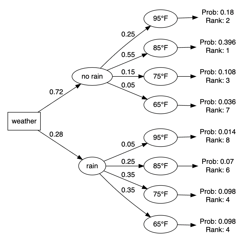
Next steps
This approach works with tree diagrams of any size, although adding scenarios with many branch levels will quickly become challenging to decipher. Some things we could also consider:
- Enhance the script to calculate and display payoff amounts by branch as well as generate overall expected value figures.
- Add formatting options such as color, font type, and font size for the visual.
- Turn the data frame manipulation into its own function that will return all conditional probabilities. This could be especially useful as the number of branches grows larger.
Inspiration
All of the code above was built on top of approaches found in the resources below:
Related Courses
Related Learning Paths
5 Courses
7 Months
Tidyverse Skills for Data Science in R