
Must know time-series analysis techniques for data analysts
9 de Abril de 2023 by Avi Kumar TalaviyaIntroduction
Time-series analysis is a crucial skill for data analysts and scientists to have in their toolboxes. With the increasing amount of data generated in various industries, the ability to effectively analyze and make predictions based on time-series data can provide valuable insights and drive business decisions.
In this article, we will understand various methods and techniques for time-series analysis, from important statistical methods to advanced machine-learning techniques. We will cover topics such as time-series decomposition, forecasting, time-series data pre-processing, and time-series data visualizations. Whether you are new to time-series analysis or looking to expand your knowledge, this article will provide a comprehensive guide to help you understand the most important concepts and tools for analyzing time-series data.
Table of contents:
- Time-series decomposition
- Time-series data analysis and visualization
- Forecasting using ARIMA models
- Stationarity test using statsmodels library
- Conclusion
1. Time series decomposition
The time-series data can be modeled as an addition or product of trend, seasonality, cyclical, and irregular components. The additive time-series model is given by
Yt = Tt + St + Ct + ItThe multiplicative time-series model is given by
Yt = Tt x St x Ct x ItWhere Tt = Trend component, St = Seasonality, Ct = cyclical component, and It = irregular component.
Let’s look at a code example of time series decomposition
from statsmodels.tsa.seasonal import seasonal_decompose

ts_decompose = seasonal_decompose(np.array(wsb_df['Sale Quantity']),
model='multiplicative',
period=12)

ts_decompose.plot()

plt.show()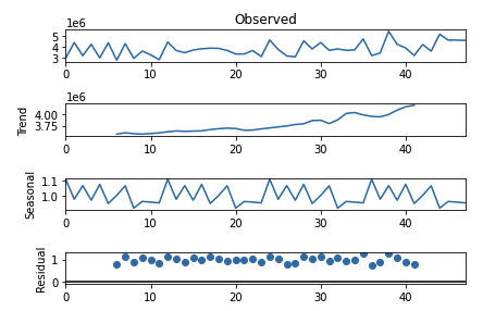
In this example, we first load the time-series data into a pandas DataFrame. We then use the seasonal_decompose function from the statsmodels library to decompose the time-series data into its trend, seasonality, and residual components. The model argument is set to 'multiplicative' to indicate that the seasonality component is multiplicative. Finally, we use the plot method to visualize the decomposition, and the show function from the matplotlib library to display the plot.
2. Time series data analysis and visualization
In this section, we will look at some of the data analysis and visualization techniques for a time-series dataset. we will take an example of a stock price dataset.
Comparative analysis of the stock prices of companies within the same industry
Comparative analysis of stock prices refers to comparing the performance of one or more stocks in a given market or industry over a specific period. The goal of this analysis is to understand how stocks are performing relative to each other and to identify trends, patterns, and relationships between them.
There are multiple methods for conducting a comparative analysis of stock prices which includes time-series analysis of stocks and commodities to compare trends, and seasonality; comparison of financial metrics like Return on investment (ROI), Price-to-earnings ratio (RoE) along with statistical analysis and visualization techniques.
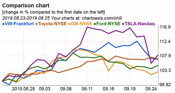
Growth of the stock prices over 5 years
The growth of stock prices refers to the increase in the value of a stock over some time. It is an important metric for investors to consider when making investment decisions, as it can indicate the potential return on investment (ROI).
The commonly used formula for calculating the growth of stock price is as below:
Rate of return = (Ending price — Starting price) / Starting priceLet’s look at python implementation to calculate the growth of stocks and then visualize the rate of growth for different stocks using matplotlib libraries.
3. Forecasting using ARIMA models
ARIMA (AutoRegressive Integrated Moving Average) models are a class of time-series forecasting models that are commonly used for modeling and predicting future values of time-series data. ARIMA models capture the autoregressive element, the difference element, and the moving average element of time-series data to make predictions.
The AR element of the model captures the dependence between the current value and previous values in the time-series data, while the MA element captures the dependence between the current value and residual errors. The ‘I’ element, also known as the difference element, is used to make a non-stationary time-series data stationary by converting it into its first differences.
1. Developing forecasting model using AR component
First, we will load the sales dataset from kaggle.
vim_df = pd.read_csv("/kaggle/input/vimanaaircraftdataset/vimana.csv")

vim_df.plot(kind='scatter', x='Month', y='demand')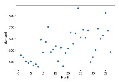
After loading the dataset, we will plot the autocorrelation plots to find out the optimal lags of the AR and MA elements.
from statsmodels.graphics.tsaplots import plot_acf, plot_pacf

# show the autocorelation upto lag 20

acf_plot = plot_acf( vim_df.demand, lags=20)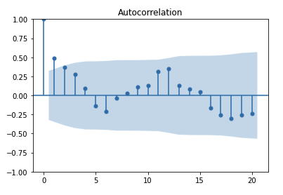
# plot the partial autocorrelation plot
pacf_plot = plot_pacf(vim_df.demand, lags=17)
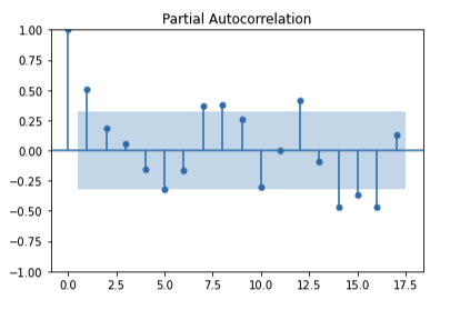
In the above plots, The shaded area represents the upper and lower bounds for critical values, where the null hypothesis cannot be rejected(the autocorrelation value is 0). So, it can be observed from the above plots that the null hypothesis is rejected only for lag=1.
Now, let’s build an AR model using the statsmodels library. ‘tsa’ module of the statsmodels library provides ARIMA class to develop various time-series models.
# we will build AR model using p=1 only.

from statsmodels.tsa.arima.model import ARIMA

# AR model with an order of (1,0,0)

arima = ARIMA(vim_df.demand[:30].astype(np.float64), order=(1,0,0))

ar_model = arima.fit()

ar_model.summary()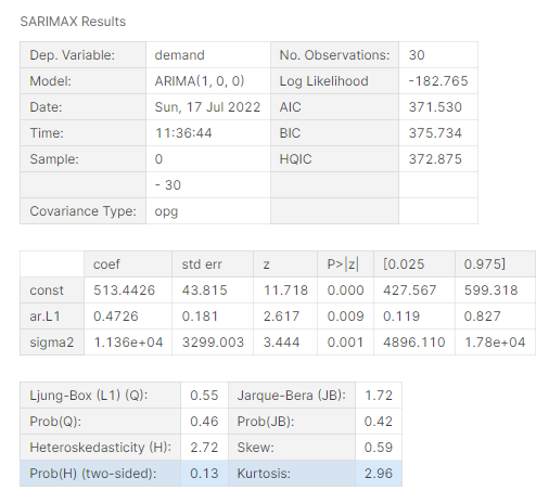
The above result shows the coefficients and P-values of the AR model. We can see that p-values of the all the coefficients are less than 0.05. So it is statistically significant. now we can use the above forecast of the future values using this model.
# forcast on new data which from 31 to 37

forecast_31_371 = ar_model.predict(30,36)

forecast_31_371
Output:
30   480.15
31   497.71
32   506.01
33   509.93
34   511.78
35   512.66
36   513.07

Name: predicted_mean, dtype: float64
Similarly, we can develop a model using ARIMA components.
2. Developing forecasting model using ARIMA components
To develop the ARIMA model, we will keep the order of the model as (1,1,1) which consists of autoregressive, difference, and moving average elements.
# let's build ARIMA model with p,d,q = (1,1,1)

arima = ARIMA(vim_df.demand[0:30].astype(np.float64), order=(1,1,1))

arima_model = arima.fit()

arima_model.summary()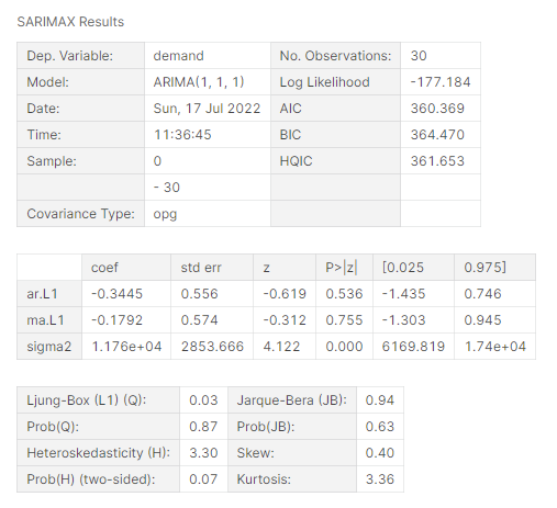
It’s important to note that choosing the right order of the AR, I, and MA elements is critical for the accuracy of the ARIMA model. One common method for selecting the right order is to use a process known as grid search, which involves fitting ARIMA models with different combinations of AR, I, and MA elements to the data and choosing the combination that provides the best fit.
4. Stationarity test using statsmodels library
The AR and MA models can only be used if the time series is stationary. The I elements help to build forecasting models on non-stationary time series. ARIMA models are used when the time-series data is non-stationary. Time-series data is called stationary if the mean, variance, and covariance are constant over time.
The main function of the I element t is to convert a non-stationary time series into a stationary time series. To verify the stationarity of the time series we can do Dicky-fuller test using the statsmodels library.
We can set up the null hypothesis and alternate hypothesis as below to test dicky-fuller test.
H0: Time series is non-stationary

Ha: Time series is a stationary
If the p-value is less than 0.05 then we will reject the null hypothesis and accept the alternative hypothesis.
from statsmodels.tsa.stattools import adfuller

def adfuller_test(ts):

    adfuller_result = adfuller(ts, autolag=None)

    adfuller_out = pd.Series(adfuller_result[0:4], index=['Test Statistic', 'p-value', 'Lags Used', 'Number of Observations Used'])

    print(adfuller_out)

# call the using with input of the time-series data

adfuller_test(store_df1.demand)
Output:
Test Statistic                 -1.65
p-value                         0.46
Lags Used                      13.00
Number of Observations Used   101.00

dtype: float64
The above output shows, the p-value is much greater than 0.05, hence we cannot reject the null hypothesis. This indicatoes that our time series is non-stationary.
As the time series is non-stationary, we have to find the difference(I) component that makes the time series stationary before modeling using ARIMA modeling.
I am attaching project notebooks and dataset sources if you want a more detailed explanation of the code.
- Github Repository — Click here
- Kaggle notebook — Click here
- Kaggel dataset — Click here
5. Conclusion
In conclusion, as a data analyst, an understanding of time-series analysis techniques is essential for making informed decisions and forecasts based on historical data. From pre-processing techniques, like handling missing values to advanced modeling methods, like ARIMA and machine learning algorithms, time-series analysis provides a wealth of tools and techniques for understanding and predicting the behavior of time-series data. Do check out some of the courses listed on this web page to learn ARIMA modeling and other time-series analysis techniques.
Cursos relacionados
26 horas
Intermedio
62.753